Linear regression in supervised learning

Oct 10, 2022Arkar Kaung Myat

PythonML

I am gonna be talking about linear regression and how gradient descent algorithms can be used to get the best outcome of our model.

When I started learning machine learning, the term - linear regression - was the very first topic that I heard a lot. My first familiarity with linear regression was when I took the cs229 course from Standford University by Andrew Ng and lecture - 2 was about linear regression and gradient descent.

In this blog, I am gonna be talking about linear regression and how gradient descent algorithms can be used to get the best outcome of our model.

Linear regression is a type of supervised learning in machine learning where you give the data set to the algorithm with the outcome and we already have some idea of what the output might be if giving some sort of input. Then the algorithm figures out what the relationship might be between these datasets and can predict what the outcome will be,

Some example use cases of linear regression are

Predicting the house prices based on the number of rooms, area, etc.
Predicting the happiness of people based on their income
Predicting the Uber price based on the distance of the trip.

The simplest possible scenario is as follows, lets say we have

X = –1, 0, 1, 2, 3, 4
Y = –3, –1, 1, 3, 5, 7

There’s a relationship between the X and Y values (for example, if X is –1 then Y is –3, if X is 3 then Y is 5, and so on). If you have ever solved some critical thinking problems or taken part in some IQ tests, you may find out the relations between those numbers very quickly which is $Y = 2X + 1$ . Different people can find out differently. In this case, X increases by 1 in its sequence so its Y = 2X + or - something . After some tries you will find out the equation is KaTeX can only parse string typed expression. In machine learning, it's called the hypothesis, $Y = 2X + 1$ fits, the data.

Not only in linear regression, in supervised learning, we first decide the approximate y ( labels) as a linear function of x (features) decide the approximate y as

h_θ (x) = θ_0 + θ_1 x_1 + θ_2x_2

Whereas, $xi$ are the inputs and $θi$ are called weights (parameters) which we guessed in above $Y = 2X + 1$ equation.

Right now there is only one input in the equation. However, in reality, a label might depend on multiple features. For example, in the house price guessing example, the house price may depend on features like the number of rooms, area, location, and views. So we can create the hypothesis for each feature in a way like this by dropping θ and letting $x_0=1$ (known as the intercept term).

h(x)=\textstyle\sum_{i=0}^dθ_ix_i

The goal is to get close $h_θ$ as close to y ( the label in the dataset ) . We gonna try to find the best fit of $θ$ .

# Cost function

In supervised learning, we try to reduce the cost of a function by using features and labels from given data set and try to tweak the parameters to fit the data nicely.

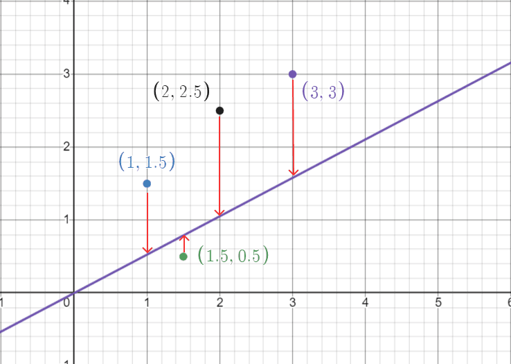
The purple line in the graph as you can see is the relation predicted by the algorithm for the first time, and the points are the data we provided to the algorithm. We can find how much the algorithm wrongfully predicted ( by subtracting the predicted value from the expected value ( the label, the red arrows ) . Also we can defined the sum of square of the error from each features and get what know as the cost function as you saw above. As $error = expected - predicted$ then $error = y - h_θ(x)$ . By using a method know as ordinary least square methods we can get the square sum of error for each feature.

J(θ)=\textstyle\sum_{i=0}^d(h_θ(x^i)-y_i)^2

If we got the error function ( cost function ) the next thing we need to consider is how to make it smaller. We gonna try to find the θ value when J(θ) is close to zero. Luckily, we can make a function smaller by using some tricks from partial derivative.

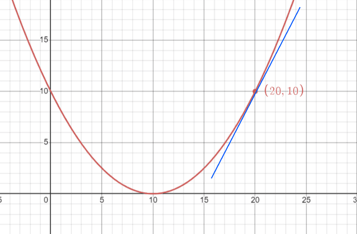
If we plot the function we now got a curve . We can use derivative of the curve to get the slope at any value for the intercept ( θ ) . Where the slope is zero means the there is no loss value and our predicted value and label are the same ( which not happen in reality ) .

# Gradient descent

We want to choose the best value of θ where $J(θ)$ is minimal. At first, we always gonna start at a wild guess by letting $θ=0$ and make changes to θ where $J(θ)$ is the smallest.

θ_j \coloneqq θ_j - \alpha\frac{∂(θ)}{∂J} J(θ)

Starting from a wild guess and repeatedly performing the update on θ for all values of j. Here, α is called the learning rate. This is a natural algorithm that controls how huge or how little we want to update the value of θ in every step of the each of j. To find out how the cost function changes according to the value θ . To get the relation between θ and the loss function.

\frac{∂}{∂θ_n}J(θ) = \frac{∂}{∂θ_n}(h_θ(x) - y_i)^2 \\ \frac{∂}{∂θ_n}J(θ) = \frac{∂}{∂θ}(\sum_{i=0}^nh_θ(x) - y_i)^2 \\ \frac{∂}{∂θ}J(θ) = \frac{∂}{∂θ}(h_θ(x) - y)^2 \\ \frac{∂}{∂θ}J(θ) = 2(h_θ(x)- y)× \frac{∂}{∂θ}(h_θ(x) - y) \\ \frac{∂}{∂θ}J(θ) = 2((θx + b)-y)× x \\ \frac{∂}{∂θ_n}J(θ_i) = \frac{2}{n}\sum_{i=0}^n( (θ_ix_i + b)- y_i)× x_i \\ \frac{∂}{∂θ_n}J(θ_i) = -\frac{2}{n}\sum_{i=0}^n( y_i -(θ_ix_i + b))× x_i

You may probably notice when I replace the value for $hθ(x)$ b is actually the y-intercept according to the slope equation, $y = mx + b$ . ( b is $θ0$ ) . We can also find the relation between b and the loss function in the same way we find for θ.

\frac{∂}{∂b_n}J(b_i) = -\frac{1}{n}\sum_{i=b}^n( y_i -(b_ix_i + b))

# In Python

The final moment of truth! in this section, I am gonna be trying to code the linear regression with the equation we formulated above. This section is I think the coolest thing that I found out in my journey. I am gonna be doing linear regression with some datasets that I found from Kaggle and trying to predict the outcome.

I am gonna be using numpy, pandas and matplotlib from python.

class LinearRegression:
    def __init__(self,x,y):
        self.data = x
        self.label = y
        self.m  = 0
        self.b = 0
        self.n = len(x)

    def fit(self, epoch, lr):
        for i in range(epoch):
            y_pred = self.m * self.data + self.b

            L_M = (-2/self.n)*sum(self.data * (self.label - y_pred))
            L_b = (-1/self.n)*sum(self.label - y_pred)

            self.m = self.m - lr * L_M
            self.c = self.b - lr * L_b

    def predict(self,inp):
        y_pred = self.m * inp + self.b
        print(self.m,self.c)
        return y_pred

In the class LinearRegression, it has two functions predict and fit. Predict function accepts two parameters epoch and lr. ( number of times we want to tweak θ to reduce the cost function.

 def fit(self, epoch, lr):
        for i in range(epoch):
            y_pred = self.m * self.data + self.b
            L_M = (-2/self.n)*sum(self.data * (self.label - y_pred))
            L_b = (-1/self.n)*sum(self.label - y_pred)
            self.m = self.m - lr * L_M
            self.c = self.b - lr * L_b

The for loop as you can see is where we adjust the value of θ according to this equation $θj \coloneqq θj - \alpha\frac{∂(θ)}{∂J} J(θ)$ we mentioned above.

L_M = (-2/self.n)*sum(self.data * (self.label - y_pred))
L_b = (-1/self.n)*sum(self.label - y_pred)

For each iteration, it finds out the $θ$ and $θ_0$ values and adjust them

self.m = self.m - lr * L_M
self.c = self.b - lr * L_b

by multiplying with the learning rate, self.c and self.m get better and better over each iteration. So our model fits with our data gradually.

# load the csv using pandas 
df = pd.read_csv('score.csv')

# extract features and labels
x = np.array(df.iloc[:,0])
y = np.array(df.iloc[:,1])

model = LinearRegression(x,y)
model.fit(1000,0.0001)
y_pred = model.predict(x)

# plot the pred results 
plt.figure(figsize = (20,6))
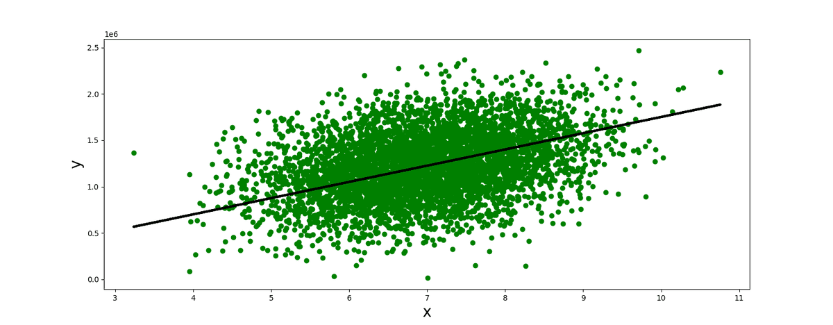
plt.scatter(x,y , color = 'green')
plt.plot(x , y_pred , color = 'k' , lw = 3)
plt.xlabel('x' , size = 20)
plt.ylabel('y', size = 20)
plt.show()

print(y_pred)

# Complete code

import numpy as np
import pandas as pd
import matplotlib.pyplot as plt

class LinearRegression:
    def __init__(self,x,y):
        self.data = x
        self.label = y
        self.m  = 0
        self.b = 0
        self.n = len(x)

    def fit(self, epoch, lr):
        for i in range(epoch):
            y_pred = self.m * self.data + self.b
            L_M = (-2/self.n)*sum(self.data * (self.label - y_pred))
            L_b = (-1/self.n)*sum(self.label - y_pred)
            self.m = self.m - lr * L_M
            self.c = self.b - lr * L_b

    def predict(self,inp):
        y_pred = self.m * inp + self.b
        print(self.m,self.c)
        return y_pred

df = pd.read_csv('score.csv')
x = np.array(df.iloc[:,0])
y = np.array(df.iloc[:,1])
model = LinearRegression(x,y)
model.fit(1000,0.0001)
y_pred = model.predict(x)

plt.figure(figsize = (20,6))
plt.scatter(x,y , color = 'green')
plt.plot(x , y_pred , color = 'k' , lw = 3)
plt.xlabel('x' , size = 20)
plt.ylabel('y', size = 20)
plt.show()
print(y_pred)

# Examples

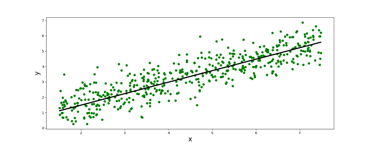
# Income vs happiness income.csv

# USA housing data set USA_Housing .csv